Jigsaw Rate Severity of Toxic Comments 14th Place Solution
UPDATE: I did an interview with Sanyam Bhutani about my solution to this competition on his Chai Time Podcast on Weights & Biases here
This blog is mostly a repost of a thread I posted on Kaggle about this competition. You can find the original thread here. The source code can be found here.
Competition Overview
The goal of this competition was to build a system which can predict how toxic online comments are. What separated this from other similar sentiment analysis tasks was that the comments were divided randomly into pairs and then the comments in each pair were ranked by annotators. For example, if an annotator receives two comments: A) “I hate you.”, and B) “That’s nice.”, they have to choose which of the two comments is “more toxic” and which is “less toxic”. The data contained some duplicate pairs which had been ranked by different annotators. This means that there were many cases of annotator disagreement, which led to inconsistent labels.
The target metric for the competition was Average Agreement with Annotators. Given a pair of texts, the system had to generate a score for each text, and if it generated a higher score for the text labelled by the annotator as “more toxic” then it would receive 1 point, otherwise 0. The final score was then the total number of points divided by the total number of text pairs. Since the dataset contained contradictory pairs, it was impossible to get a score of 1.0 (100% agreement with all annotators).
The test set was 200,000 pairs of comments, and the public leaderboard which is visible throughout the competition only contained 5%, or about 10,000 pairs, of the total test data. The small size of the public leaderboard meant that it was not a very reliable metric, which led lots of teams to overfit.
Another complicating factor was that we didn’t receive any training data for the competition. Instead we got a validation set, and some links to other similar toxicity-rating tasks to potentially use as extra data.
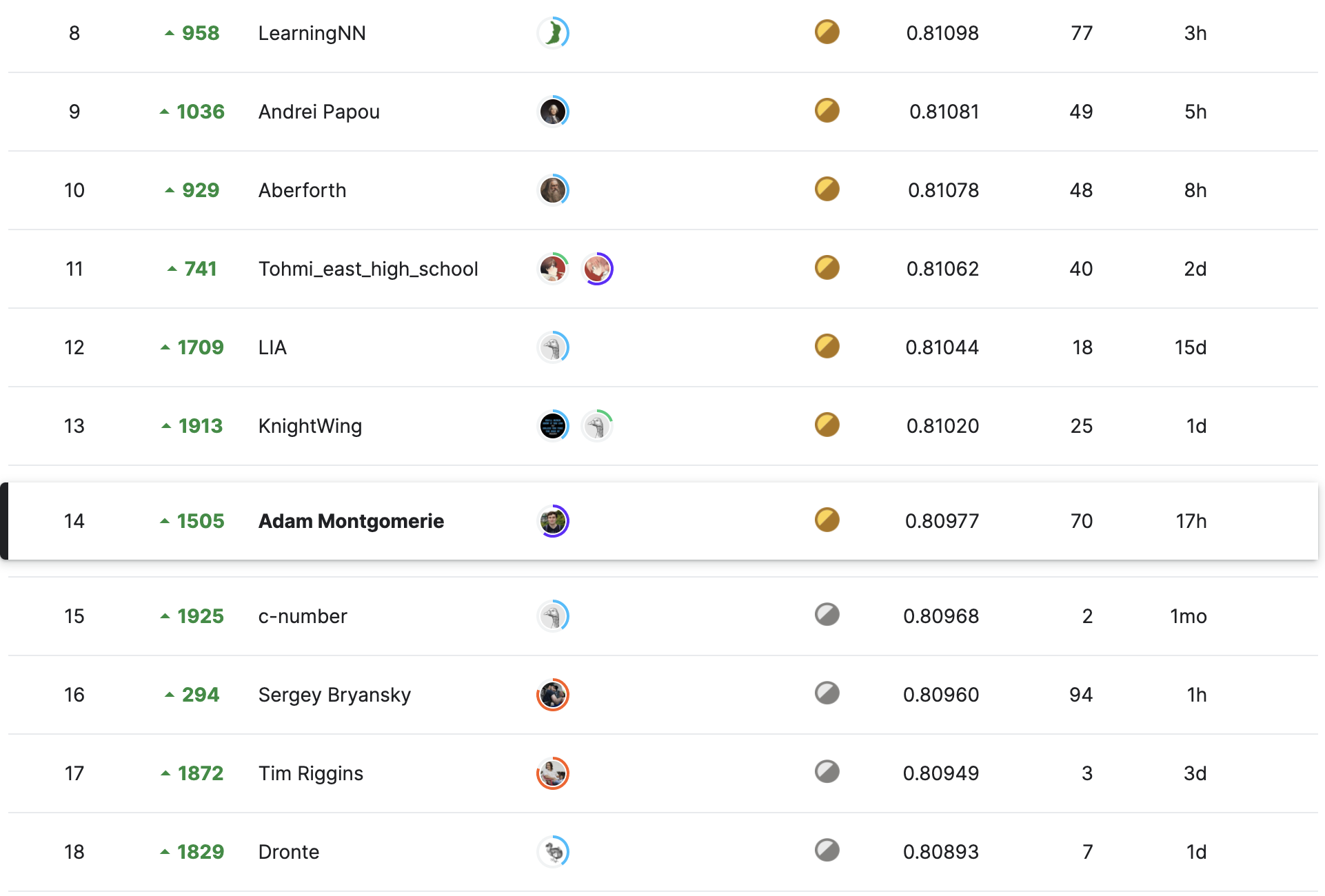
In the end I came in 14th place, just barely getting a gold medal!
Solution Overview
The public leaderboard didn’t seem very useful so my strategy was to just maximise my validation score. My final submission is a weighted mean of 6 (5-fold) transformers. It was both my highest CV (Cross Validation score) and highest private LB score, so I’m glad I trusted my CV this time.
Data
I tried to include as many different datasets as I could. For training I used:
- the validation set
- jigsaw 1: the data from the first jigsaw competition
- jigsaw 2: the data from the second jigsaw competition
- ruddit: the data from Ruddit: Norms of Offensiveness for English Reddit Comments
- offenseval2020: the data from OffensEval 2020: Multilingual Offensive Language Identification in Social Media. This dataset was uploaded to haggle by @vaby667 here
CV strategy
I used the Union-Find method by @columbia2131 to generate folds that didn’t have any texts leaked across folds. I didn’t use majority voting or any other method of removing disagreements from the data, as I thought this would just make the validation set artificially easier and less similar to the test data.
Training
Loss
I used Margin Ranking Loss to train with the validation data, and tried both Margin Ranking and MSE (Mean Squared Error) with the other datasets. It was fairly easy to create large amounts of ranked paired data from the extra datasets, but I didn’t find that this improved performance over just training them directly on the labels with MSE loss, and also required lower batch sizes.
Evaluation
When fine-tuning on the extra datasets, I computed average agreement with annotators on the validation set at each evaluation, and used early stopping. I trained for multiple epochs on the small datasets (jigsaw 1 and ruddit), evaluating once an epoch. For the large datasets (offenseval and jigsaw 2) I usually only trained for 1 epoch, evaluating every 10% the epoch’s steps.
When training on the validation data, I trained 5 models, using 4/5 folds for training and the remaining fold as validation for each one. I computed the CV at each epoch and used the model weights from the epoch that had the highest CV.
I had original started out using fold-wise early stopping, but I discovered that this leads to overly optimistic CV scores.
Multi-stage fine-tuning
I found that taking a model I had already fine-tuned, and fine-tuning it on another dataset improved performance. This worked across multiple fine-tuning stages. The order that worked best was to start by fine-tuning on the larger, and lower scoring, datasets first, and then on the smaller ones after.
For example:
- fine-tune a pretrained model on offenseval (validation: ~0.68)
- use #1 to fine-tune on jigsaw 2 (validation ~0.695)
- fine-tune #2 on jigsaw 1 (validation ~0.7)
- fine-tune #3 on ruddit (validation ~0.705)
- fine-tune 5 folds on the validation data, using #4 (CV: 0.71+)
Hyperparameters
I started out training most of the base-sized models with 1e-5 on earlier fine-tuning stages and reduced to 1-6 on the later ones. I used 1e-6 and then 5e-7 on the larger models. At each stage I also used warmup of 5% and linear LR decay. Even with mixed precision training, I could only fit batch size 8 on the GPU with the large models, so I used gradient accumulation to simulate batch sizes of 64.
Models
Here’s a table of model results.
| base model | folds | CV | final submission |
|---|---|---|---|
| deberta-v3-base | 5 | 0.715 | yes |
| distilroberta-base | 5 | 0.714 | yes |
| deberta-v3-large | 5 | 0.714 | yes |
| deberta-large | 10 | 0.714 | yes |
| deberta-large | 5 | 0.713 | yes |
| rembert | 5 | 0.713 | yes |
| roberta-base | 5 | 0.711 | no |
| roberta-large | 5 | 0.708 | no |
Notes:
- I mostly stuck to using roberta and deberta variants because they always perform well. If I had had more time I would’ve tried some others, but I spent most of the time trying out different combinations of datasets.
- The reason I tried rembert was because I wanted to make use of the multilingual jigsaw 3 data. I wasn’t able to get any improvement from including the extra data, but I was still able to get reasonably good performance out of rembert.
- Deberta-large (v1) is in there twice because I did an experiment with a 10 fold model which turned out quite well. I didn’t want to keep training 10 fold models though because it took too long.
- I think all of the large models are slightly under-trained. Training on large datasets like offenseval and jigsaw 2 took over 24 hours so my colab instances timed-out.
Ensembling
My final submission was a weighted mean of 6 models which were selected from a pool of models by trying to add each of them to the ensemble one at a time, tuning the weights with Optuna for each combination of models, and greedily selecting whichever model increased the OOF score the most. This was repeated until the OOF score stopped improving. My best score was 0.7196.
Interestingly, the highest weighted models ended up being deberta-large and rembert, despite those having lower CV scores.
Things which didn’t work
The measuring hate speech dataset
The Measuring Hate Speech dataset by ucberkeley-dlab seemed like it was going to be useful, but the labels didn’t seem to match the annotations in the validation set for this competition very well. I was unable to get more than 0.656 with this data.
Binary labels
I wanted to try to make use of the binary labelled data too (jigsaw 3 and toxic tweets). I tried fine-tuning on these datasets, and used the model’s predicted probability of the positive class as an output for inference and evaluation. I was able to get 0.68 on the validation set with this method, but I found that it didn’t chain together with my multi-stage fine-tuning approach as I had to modify the last layer of the model to switch between regression and classification tasks.
TF-IDF with linear models
This method was used by a large number of competitors in this competition, but it seems to have mostly been used to overfit the small public LB. I experimented with it a little bit, but wasn’t able to get anything over 0.7 on the validation set so I gave up on it.
Word vectors with linear models
I tried encoding each comment as the average of spaCy word vectors, and using this as an input into various linear models. It did about as well as TF-IDF.
Improvements
As I’ve already mentioned, I think my large models are under-trained due to GPU limitations. I was surprised by how much rembert helped the ensemble, so think I could’ve made a stronger ensemble by choosing some more diverse model architectures instead of focusing on deberta and roberta so much.
Overall, I’m quite happy with how this competition came out. I feel very lucky to have got a gold medal this time!