Classifying Heavy Metal Subgenres with Mel-spectrograms
Distinguishing between broad music genres like rock, classical, or hip-hop is usually not very challenging for human listeners. However being able to tell apart the subgenres of these broad categories is not always so simple. Someone who is not already a big fan of house music probably won’t be able to distinguish deep house from tech house for example. The subtle differences between subgenres only become apparent when you become a more experienced listener. Training a neural network to classify music genres is not a new idea, but I thought it would be interesting to see if one could be trained to classify subgenres on a more precise level.
I got the original idea from reading a blog post by Priya Dwivedi. In the blog, music samples are converted to mel-spectrograms, and then fed into neural networks with both convolutional and recurrent layers in order to generate a prediction. I decided to try a similar method, but with the goal of classifying subgenres instead of top-level genres. In order to achieve this, I needed to build a dataset.
Data Collection
In the last post I discussed collecting track data and mp3 samples from Spotify to generate a dataset. I collected track data for 100,000 songs using Spotipy and downloaded a 30-second track sample for each one. The data collection strategy was the one referred to as Artist Genres as Labels in my previous post.
I decided to focus mostly on a single parent genre in order to limit the number of possible subgenres to prevent the number of classes getting out of hand. I chose metal since I’m a fan of the genre and feel confident classifying metal subgenres. I made a list of 20 subgenres, mostly from metal but also including subgenres from punk, rock, and hardcore where those genres border on metal.
For comparison I also collected another dataset of top level genres like classical, rock, and folk. This dataset is smaller, at only about forty thousand examples, and contains only ten classes.
After collecting track data from artists for all of the subgenres and downloading track samples for them, I converted the samples from mp3 files to mel-spectrogram pngs. A spectrogram is a visual representation of sound frequencies over time. Usually the Y-axis is decibels and the X-axis is time. Mel-spectrograms are a type of spectrogram where the Y-axis uses the Mel scale. This means that it has been rescaled to more accurately reflect the ways that humans hear sounds.
Here’s some examples of processed mel-spectrograms which I generated:
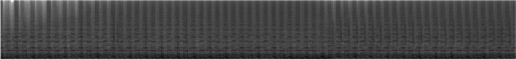 Techno
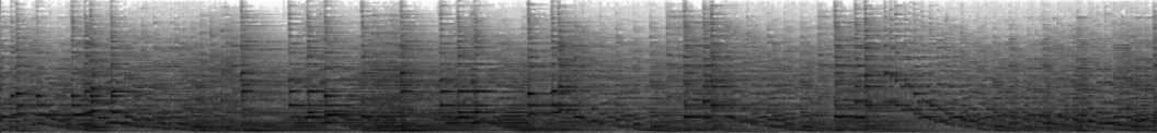 Classical
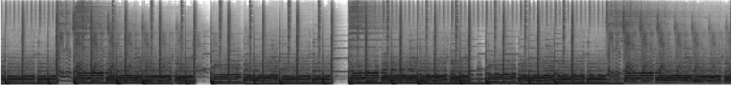 Jazz
Jazz
The vertical axis is frequency, and the horizontal axis is time (thirty seconds of each track). I didn’t label or colourise these images because they were originally meant for a neural network rather than a human audience. At a glance, we can see some differences. Techno is very uniform, whereas jazz is quite irregular. Classical seems to softly change over time, whereas jazz appears to more suddenly change.
Architecture
The model is based on Convolutional Recurrent Neural Networks for Music Classification by Keunwoo Choi et al. The model includes both convolutional layers and recurrent layers, allowing us to take advantage of the benefits of both.
CNNs
Convolutional Neural Networks (CNNs) can be used to capture both low and high-level features of images, and are a standard part of image-recognition systems. In convolutional layers, filters are passed over inputs to generate feature maps. A feature map is like the encoded input image, but can be smaller in size while retaining important information and spatial relationships from the original image. A more detailed description of CNNs can be found in this blog.
Convolutional layers can be stacked to capture information from an image with varying levels of abstraction. Earlier layers might capture low level features like edges or corners, and later layers might instead detect discrete objects like faces or cars. This is useful in the case of classifying spectrograms as, by stacking some convolutional layers, we can capture both the low level relationships between adjacent pixels representing sound at various frequencies, and the high level structure of the spectrogram representing the piece of music as a whole.
RNNs
Recurrent Neural Networks (RNNs) are used to capture sequential relationships in input data, for example the relationships between words in text or between data points in a time series. This is achieved by maintaining a hidden state inside each layer which acts as a “memory” of previous inputs. The hidden state is combined with the new input to produce an output and a new hidden state. This process can be repeated as many times as necessary until the whole sequence has been processed. In theory, this means that the final output should include information from not just the final element of the sequence but all the previous elements too.
In practice however, standard RNNs’ ability to “memorise” previous inputs is fairly limited, and they are ineffective at processing long sequences. Long Short-Term Memory networks (LSTMs) attempt to resolve this issue by introducing a cell state and a more complex system for determining what information is kept and what is discarded. This allows the network to learn from more long-term dependencies. Here’s a great blog which discusses RNNs and LSTMs in more detail. In the Convolutional Recurrent Neural Network (CRNN) model, a Gated Recurrent Unit (GRU) is used instead of an LSTM, which is a slightly more lightweight version which retains most of the advantages.
The reason for introducing an RNN component into the network is that spectrograms are a representation of time series data: in this case sound at various frequencies over time. By feeding the spectrogram from left to right into a GRU, we can hopefully capture some of the sequential nature of a piece of music.
CRNN
The CRNN model is simply a CNN stacked on an RNN. The intuition for using these things together is that spectrograms can be viewed both as images and as sequences. Using a CNN allows us to process the spectrogram as an image, and using an RNN allows us to process it as a time sequence.
To generate a prediction, an input image (or batch of images) is encoded and passed into the network. The image is first passed into the CNN sub-network, which is made up of 4 blocks. Each block contains a convolutional layer, batch normalisation, a ReLU activation function, and finally a max-pooling layer. Each block gradually reduces the dimensions of the input image until the output of the final block is a feature map of only one pixel in height and twenty in width (fifteen in the original paper, but my images were wider to begin with). This feature map is then used as an input sequence into the RNN sub-network, where each pixel is an element of the sequence. The sequence is fed into a two-layer GRU, followed by a dense layer. The final prediction is generated by passing the RNN output through a dense layer of width equal to the number of genre classes we have.
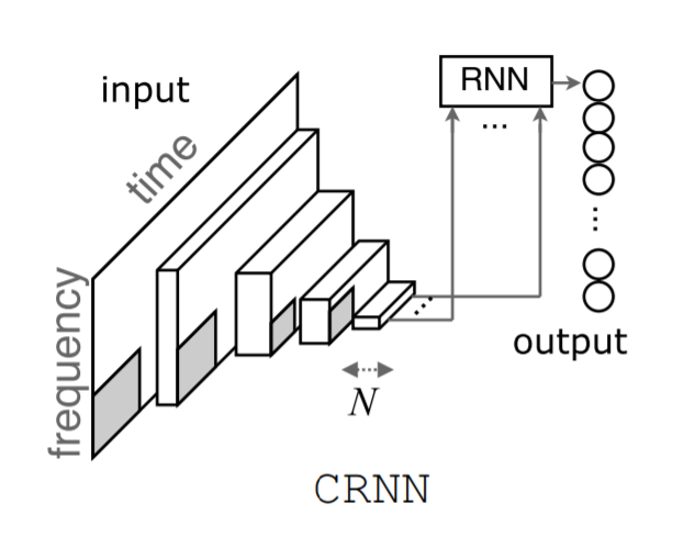
Image taken from *Convolutional Recurrent Neural Networks for Music Classification by Keunwoo Choi et al.*
The image shows the input spectrogram on the left. We can see that it is reduced in size gradually by being passed through four convolutional layers. N represents the number of feature maps. We can see that the frequency dimension is reduced to one, so we are just left with a sequence over the time dimension, which is passed to the RNN section. The circles on the right show the possible labels that can be selected from.
My PyTorch implementation of this model can be found here.
Training & Results
The datasets were split into 80% training and 20% test set. The model was trained over 10 epochs with a learning rate of 0.0017 (after using fast.ai’s learning rate finder) on a GPU using Google Colab.
I first tried training on the smaller dataset of high-level genres first, and was able to get 80% accuracy on the test set, which is pretty good. After that, I tried training the same model on the larger metal subgenre dataset, where the test accuracy dropped to below 50%. This is understandable as, despite being two and a half times larger, the dataset has twice as many classes, and the classes are much more similar to each other.
Including Tabular Data
Although the main data source in this project was the 30-second track samples, I was also able to collect some other track data from the Spotify API. This tabular data includes features like track length, mode, key, number of sections, and some Spotify-generated metrics like valence, danceability, and acousticness.
I guessed that these values also have some predictive power, so I tried including them into the model to see if it improved predictions: I found that it did!
How it works is, in addition to the architecture described in the previous section, tabular data relating to a given track sample is encoded and fed into a dense layer. It then goes through a ReLU and another dense layer. The output of this small feed-forward network is concatenated with the output of the RNN and used to make the final prediction.
I retrained the model with this modification and extra source of data, and found that this significantly improved the accuracy from about 50% to 62% top-one accuracy.
An implementation of this version of the model can be found here.
Confusion Matrix
I generated a confusion matrix from each of the trained models to see which genres were most commonly mixed up. I hypothesized that closely related subgenres would be much more likely to be confused. For example, the metal subgenre dataset has “death metal”, “deathcore”, and “melodic death metal” as separate classes. These are distinct subgenres, but musically do borrow a lot from each other.
Here’s the confusion matrix:
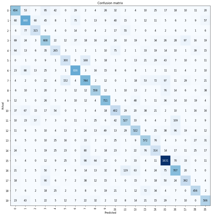
Here’s a key for the labels:
{'black metal': 0,
 'death metal': 1,
 'deathcore': 2,
 'doom metal': 3,
 'folk metal': 4,
 'glam metal': 5,
 'grindcore': 6,
 'hard rock': 7,
 'hardcore': 8,
 'industrial metal': 9,
 'melodic death metal': 10,
 'metalcore': 11,
 'nu metal': 12,
 'power metal': 13,
 'progressive metal': 14,
 'punk': 15,
 'screamo': 16,
 'stoner rock': 17,
 'symphonic metal': 18,
 'thrash metal': 19}
Completely contrary to my expectations, the most confused subgenres were:
- hard rock with industrial metal
- grindcore with progressive metal
- stoner rock with industrial metal
I would’ve imagined that perhaps hard rock and stoner rock would get mis-labelled as each other, but instead the model confused them both with industrial metal! This is perhaps partly a dataset problem. The tag “industrial” is thrown around quite casually and sometimes assigned to bands that don’t really fit, so it’s possible that some bands were mis-labelled in Spotify’s database.
But what’s even more surprising is the confusion between grindcore and progressive metal. Grindcore is very fast but usually pretty straight forward music, with songs that rarely last more than two minutes. Progressive metal on the other hand often has songs that last ten minutes or more, and features all sorts of tempo and mood changes as well as other things.
That these two genres were confused shows that the features the model is picking out when classifying are not the same kind of things that a human picks out, because even someone who has never listened to grindcore or progressive metal before would be able to tell the difference. Here’s an example of grindcore and here’s some prog metal in case you want to try comparing them for yourself.
Conclusions
I would consider this project a modest success as the model was clearly able to find some patterns in both datasets and make accurate predictions of high-level genres and subgenres with 80% and 60% accuracy respectively. My assumption that subgenres would be more difficult to classify than broad genres was also confirmed. On the other hand, the confusion matrix shows that the things that I thought would be difficult to classify didn’t necessarily turn out to be, and the model struggled with some things that would seem obvious to a human listener (at least if the given human is a metalhead).
Multi-Class Versus Mult-Label Classification
In this project, the classification task was framed as a multi-class problem; i.e. there is a set of possible classes from which one correct answer must be chosen. In hindsight, perhaps a multi-label classifier would have been better. Multi-label here means that the model can select more than one correct answer from the set of classes.
The reason that this would be preferable is that it would allow us to deal with subgenre edge cases more easily. By this I mean cases where a track or artist only partially fits within a genre category. It’s not uncommon for music to cross genre boundaries and mix several styles together. In cases like these, the classifier I trained is forced to pick whichever label seems most appropriate. But if we allow it to pick more than one label it will be able to list all the genres which feature in the sample.
This issue is exacerbated by some bad subgenre choices on my part. As previously mentioned, I included both “death metal” and “melodic death metal” as classes as I think of them as distinct subgenres. However, as the name suggests, “melodic death metal” is basically a type of death metal. This means that any time we label something as melodic death metal, we are also implicitly labelling it as death metal, as that is the parent genre.
When we take into account top-five accuracy instead of just top-one, the metal subgenre classifier’s accuracy shoots up to 92%. This shows that in most cases it is recognising the specified “correct” label even when it gets it wrong. There are many tracks in the dataset that could have multiple correct labels. I would probably have the same problem if I were asked to classify some pieces of music and told that I’m only allowed to pick one label. There are many cases where we need at least two or three labels to fully describe what’s going on. If I were to do this again, or develop this project further, I’d keep a set of labels of variable length for each track sample, and allow the model to pick more than one class when making predictions.